Image processing with Python and SciPy

Given that NumPy provides multidimensional arrays, and that there is core support through the Python Imaging Library and Matplotlib to display images and manipulate images in the Python environment, it's easy to take the next step and combine these for scientific image processing. As part of our short course on Python for Physics and Astronomy we begin by exploring how Python handle image input and output

Python Imaging Library - PIL

Before we get into the broad area of image processing in Python, there is a caveat for users PIL in Python 3. The essential Python Imaging Library (PIL) is not yet completely compatible with new version of Python. Consequently the FITS tools we will need for astronomical image processing are also currently only supported in the mature versions of Python 2. The comments that follow are based on Python 2.7.

PIL provides functions to manipulate images, including reading, modifying and saving in various standard image formats. Its functions are documented in an on-line manual with a tutorial, and in this handy pdf guide.

As a simple starting example, suppose you have an image that was taken with the camera turned so that "up" is to the side when the image is displayed. Here's how you would rotate an image 90 degrees.

import Image as pil

parser= argparse.ArgumentParser(description = 'Rotate a png image 90 degrees')

if len(sys.argv) == 1:
  sys.exit("Usage: png_image_rotate file.png ")
  exit()
elif len(sys.argv) == 2:
  infilename = sys.argv[1]
else:
  sys.exit("Usage: png_image_rotate file.png ")
  exit() 

myimage = pil.open(infilename)

mirror = myimage.transpose(pil.ROTATE_90)
outfilename = os.path.splitext(os.path.basename(infilename))[0]+'_r90.png'
mirror.save(outfilename)

The first part of this is standard form to get the image name on the command line and make it available to the program. The PIL is imported with Image, and appears in the code as "pil". This is an amazingly short program, because in opening the image the library handles all the conversions in formatting and stores the image internally so that you refer to it only by the name assigned when it is loaded. We operate on the image with the transpose function, which has an argument that controls what it does. Here we rotate the image 90 degrees, and then save it to a file with a new name. The saving operation converts the internal data back to the file format set by the extension used in the file name.

You can transpose an image left-right with

mirror = myimage.transpose(pil.FLIP_LEFT_RIGHT)

or do both in one step with

mirror = myimage.transpose(Image.FLIP_LEFT_RIGHT).transpose(pil.ROTATE_90)

Processing is not limited to "PNG" files, though that file type is preferred because it is not a lossy storage option. Python reads and writes "jpg" files too. While PIL provides some essential functionality, for more practical uses in astronomy we need to read Flexible Image Transport or "FITS" files, and to enable numerical work on images in SciPy.

SciPy image processing

SciPy can read jpg and png images directly, without using PIL. With SciPy images are stored in numpy arrays, and we have direct access to the data for uses other than visualization.

import numpy as np
import matplotlib.pyplot as plt
from scipy.misc import imread, imsave

image_data = imread('test.jpg').astype(np.float32)
print 'Size: ', image_data.size
print 'Shape: ', image_data.shape

scaled_image_data = image_data / 255.

plt.imshow(scaled_image_data)
plt.show()

exit()

For our 512x512 color test image, this returns

Size:  786432
Shape:  (512, 512, 3)

because the image is 512x512 pixels and has 3 planes -- red, green, and blue. When SciPy reads a jpg or png image it will separate the colors for you. The "image" is a data cube. In the imread line we control the data type within the Python environment. Of course the initial data is typically 8 bits for color images from a cell phone camera, 16 bits for scientific images from a CCD, and perhaps 32 bits for processed images that require the additional dynamic range.

We can display images with matplotlib.pyplot using imshow() --

imshow(X, cmap=None, norm=None, aspect=None, interpolation=None,
  alpha=None, vmin=None, vmax=None, origin=None, extent=None, **kwargs)

where "X" is the image array. If X is 3-dimensional, imshow will display a color image. Matplotlib has a tutorial on how to manage images. Here, we linearly scale the image data because for floating point imshow requires values between 0. and 1., and we know beforehand that the image is 8-bits with maximum values of 255.

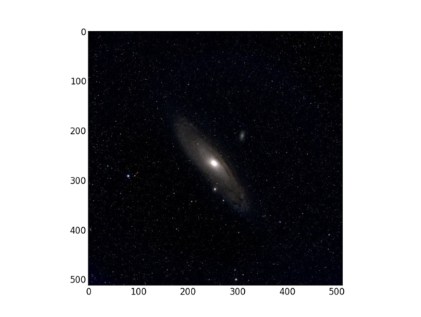
Here's what a single test image displayed from this program looks like in Python.

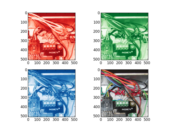
We can slice the image data to see each color plane by creating new arrays indexed from the original one.

import numpy as np
from scipy.misc import imread, imsave
import pylab as plt

image_data = imread('test.jpg').astype(np.float32)
scaled_image_data = image_data / 255.

print 'Size: ', image_data.size
print 'Shape: ', image_data.shape
  
image_slice_red =  scaled_image_data[:,:,0]
image_slice_green =  scaled_image_data[:,:,1]
image_slice_blue =  scaled_image_data[:,:,2]

print 'Size: ', image_slice_0.size
print 'Shape: ', image_slice_0.shape

plt.subplot(221)
plt.imshow(image_slice_red, cmap=plt.cm.Reds_r)

plt.subplot(222)
plt.imshow(image_slice_green, cmap=plt.cm.Greens_r')

plt.subplot(223)
plt.imshow(image_slice_blue, cmap=plt.cm.Blues_r)  

plt.subplot(224)
plt.imshow(scaled_image_data)  

plt.show()

For a colorful image you will see the differences between each slice --

Astronomical FITS files with PyFITS

PyFITS is available from the Space Telescope Science Institute, and can be added easily to a Python installation that already has NumPy and SciPy. As of January 2013, the current version 3.1.1 of PyFITS supports all the functions needed to manage image and table data in the standard Flexibile Image Transport System (FITS) files of astronomy.

Once a FITS file has been read, the header is accessible for reading, and the image data are available in a numpy array. To read and display a file we would

import os
import sys
import argparse
import numpy as np
import pyfits
import matplotlib 
import matplotlib.pyplot

# Define a function for making a linear gray scale
def lingray(x, a=None, b=None):
 """
 Auxiliary function that specifies the linear gray scale.
 a and b are the cutoffs : if not specified, min and max are used
 """
 if a == None:
         a = np.min(x)
 if b == None:
         b = np.max(x)
 return 255.0 * (x-float(a))/(b-a)

# Define a function for making a logarithmic gray scale
def loggray(x, a=None, b=None):
 """
 Auxiliary function that specifies the logarithmic gray scale.
 a and b are the cutoffs : if not specified, min and max are used
 """
 if a == None:
         a = np.min(x)
 if b == None:
         b = np.max(x)          
 linval = 10.0 + 990.0 * (x-float(a))/(b-a)
 return (np.log10(linval)-1.0)*0.5 * 255.0

# Provide information to the argparse routine if we need it
parser= argparse.ArgumentParser(description = 'Display a
  fits image')

# Test for command line arguments
if len(sys.argv) == 1:
 sys.exit("Usage: display_fits infile.fits ")
 exit()
elif len(sys.argv) == 2:
 infits = sys.argv[1]
else:
 sys.exit("Usage: display_fits infile.fits ")
 exit() 

# Open the fits file and create an hdulist
inhdulist = pyfits.open(infits) 

# Assign the input header in case it is needed later
inhdr = inhdulist[0].header

# Assign image data to a numpy array
image_data =  inhdulist[0].data

# Print information about the image
print 'Size: ', image_data.size
print 'Shape: ', image_data.shape

# Show the image
new_image_data = lingray(image_data)
new_image_min = 0.
new_image_max = np.max(new_image_data)
matplotlib.pyplot.imshow(new_image_data, vmin = new_image_min, 
 vmax = new_image_max, cmap ='gray')  
matplotlib.pyplot.show()  

# Close the input image file and exit
inhdulist.close()
exit ()

Examples

For examples of Python illustrating image processing, see the examples section.

Assignments

For the assigned homework to use these ideas, see the assignments section.