Image processing with Python and SciPy

Given that NumPy provides multidimensional arrays, and that there is core support through the Python Imaging Library and Matplotlib to display images and manipulate images in the Python environment, it's easy to take the next step and combine these for scientific image processing. As part of our short course on Python for Physics and Astronomy we begin by exploring how Python handle image input and output

Python Imaging Library - PIL

Before we get into the broad area of image processing in Python, there is a caveat for users PIL in Python 3. The essential Python Imaging Library (PIL) is not yet completely compatible with new version of Python. Consequently the FITS tools we will need for astronomical image processing are also currently only supported in the mature versions of Python 2. The comments that follow are based on Python 2.7.

PIL provides functions to manipulate images, including reading, modifying and saving in various standard image formats. Its functions are documented in an on-line manual with a tutorial, and in this handy pdf guide.

As a simple starting example, suppose you have an image that was taken with the camera turned so that "up" is to the side when the image is displayed. Here's how you would rotate an image 90 degrees.

import Image as pil

parser= argparse.ArgumentParser(description = 'Rotate a png image 90 degrees')

if len(sys.argv) == 1:
  sys.exit("Usage: png_image_rotate file.png ")
  exit()
elif len(sys.argv) == 2:
  infilename = sys.argv[1]
else:
  sys.exit("Usage: png_image_rotate file.png ")
  exit()

myimage = pil.open(infilename)

mirror = myimage.transpose(pil.ROTATE_90)
outfilename = os.path.splitext(os.path.basename(infilename))[0]+'_r90.png'
mirror.save(outfilename)

The first part of this is standard form to get the image name on the command line and make it available to the program. The PIL is imported with Image, and appears in the code as "pil". This is an amazingly short program, because in opening the image the library handles all the conversions in formatting and stores the image internally so that you refer to it only by the name assigned when it is loaded. We operate on the image with the transpose function, which has an argument that controls what it does. Here we rotate the image 90 degrees, and then save it to a file with a new name. The saving operation converts the internal data back to the file format set by the extension used in the file name.

You can transpose an image left-right with

mirror = myimage.transpose(pil.FLIP_LEFT_RIGHT)

or do both in one step with

mirror = myimage.transpose(Image.FLIP_LEFT_RIGHT).transpose(pil.ROTATE_90)

Processing is not limited to "PNG" files, though that file type is preferred because it is not a lossy storage option. Python reads and writes "jpg" files too. While PIL provides some essential functionality, for more practical uses in astronomy we need to read Flexible Image Transport or "FITS" files, and to enable numerical work on images in SciPy.

SciPy image processing

SciPy can read jpg and png images directly, without using PIL. With SciPy images are stored in numpy arrays, and we have direct access to the data for uses other than visualization.

import numpy as np
import matplotlib.pyplot as plt
from scipy.misc import imread, imsave

image_data = imread('test.jpg').astype(np.float32)
print 'Size: ', image_data.size
print 'Shape: ', image_data.shape

scaled_image_data = image_data / 255.

# Save the modified image if you want to
# imsave('test_out.png', scaled_image_data)

plt.imshow(scaled_image_data)
plt.show()

exit()

For our 512x512 color test image, this returns

Size:  786432
Shape:  (512, 512, 3)

because the image is 512x512 pixels and has 3 planes -- red, green, and blue. When SciPy reads a jpg or png image it will separate the colors for you. The "image" is a data cube. In the imread line we control the data type within the Python environment. Of course the initial data is typically 8 bits for color images from a cell phone camera, 16 bits for scientific images from a CCD, and perhaps 32 bits for processed images that require the additional dynamic range.

We can display images with matplotlib.pyplot using imshow() --

imshow(X, cmap=None, norm=None, aspect=None, interpolation=None,
  alpha=None, vmin=None, vmax=None, origin=None, extent=None, **kwargs)

where "X" is the image array. If X is 3-dimensional, imshow will display a color image. Matplotlib has a tutorial on how to manage images. Here, we linearly scale the image data because for floating point imshow requires values between 0. and 1., and we know beforehand that the image is 8-bits with maximum values of 255.

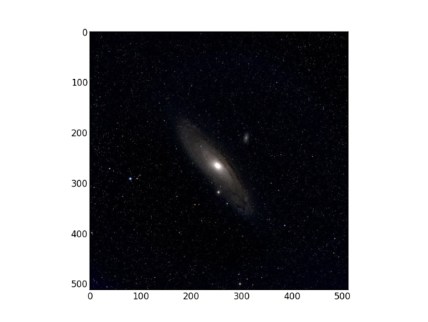
Here's what a single test image displayed from this program looks like in Python.

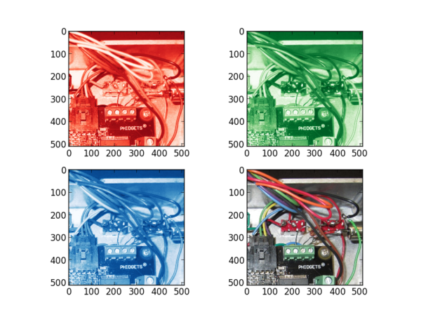
We can slice the image data to see each color plane by creating new arrays indexed from the original one.

import numpy as np
from scipy.misc import imread, imsave
import pylab as plt

image_data = imread('test.jpg').astype(np.float32)
scaled_image_data = image_data / 255.

print 'Size: ', image_data.size
print 'Shape: ', image_data.shape
  
image_slice_red =  scaled_image_data[:,:,0]
image_slice_green =  scaled_image_data[:,:,1]
image_slice_blue =  scaled_image_data[:,:,2]

print 'Size: ', image_slice_0.size
print 'Shape: ', image_slice_0.shape

plt.subplot(221)
plt.imshow(image_slice_red, cmap=plt.cm.Reds_r)

plt.subplot(222)
plt.imshow(image_slice_green, cmap=plt.cm.Greens_r')

plt.subplot(223)
plt.imshow(image_slice_blue, cmap=plt.cm.Blues_r)

plt.subplot(224)
plt.imshow(scaled_image_data)

plt.show()

For a colorful image you will see the differences between each slice --

Astronomical FITS files with PyFITS

PyFITS is available from the Space Telescope Science Institute, and can be added easily to a Python installation that already has NumPy and SciPy. As of January 2013, the current version 3.1.1 of PyFITS supports all the functions needed to manage image and table data in the standard Flexibile Image Transport System (FITS) files of astronomy.

Once a FITS file has been read, the header is accessible for reading, and the image data are available in a NumPy array. With PyFITS and NumPY you can read, extract information, modify, display and save image data.

Displaying a FITS file in Python

There are many image display tools for astronomy, and perhaps the most widely used is ds9 which is available for Linux, MacOS, and Windows, as well as in source code. It is useful to have a version on your computer when you are working with FITS images. However, sometimes we want to view an image while we are processing it in Python, and for that we could use a routine such as this one.

import os
import sys
import argparse
import numpy as np
import pyfits
import matplotlib 
import matplotlib.pyplot

Sometimes submodules are not loaded with the larger package, and we explictly ask for pyplot.

# Define a function for making a linear gray scale
def lingray(x, a=None, b=None):
 """
 Auxiliary function that specifies the linear gray scale.
 a and b are the cutoffs : if not specified, min and max are used
 """
 if a == None:
         a = np.min(x)
 if b == None:
         b = np.max(x)
 return 255.0 * (x-float(a))/(b-a)

# Define a function for making a logarithmic gray scale
def loggray(x, a=None, b=None):
 """
 Auxiliary function that specifies the logarithmic gray scale.
 a and b are the cutoffs : if not specified, min and max are used
 """
 if a == None:
         a = np.min(x)
 if b == None:
         b = np.max(x)          
 linval = 10.0 + 990.0 * (x-float(a))/(b-a)
 return (np.log10(linval)-1.0)*0.5 * 255.0

These functions may be used to rescale the data for display. Scaling can be done with a colormap, or by modifying the data before displaying. Here, we modify the data and save it in a temporary buffer for display. In a more elaborate program with a full user interface, this scaling could be done interactively.

# Provide information to the argparse routine if we need it
parser= argparse.ArgumentParser(description = 'Display a
  fits image')

The argparse function offers more flexibility than the system routines, though here we only include this for future additions.

# Test for command line arguments
if len(sys.argv) == 1:
 sys.exit("Usage: display_fits infile.fits ")
 exit()
elif len(sys.argv) == 2:
 infits = sys.argv[1]
else:
 sys.exit("Usage: display_fits infile.fits ")
 exit()

# Open the fits file and create an hdulist
inhdulist = pyfits.open(infits)

# Assign the input header in case it is needed later
inhdr = inhdulist[0].header

# Assign image data to a numpy array
image_data =  inhdulist[0].data

The header and data are now available. We'll look at header information later. For now, all we need are the values in the numpy data array. It will be indexed from [0,0] at the upper left of the data space, which would be the upper left of the displayed image.

# Print information about the image
print 'Size: ', image_data.size
print 'Shape: ', image_data.shape

For this example we use linear scaling.

# Show the image
new_image_data = lingray(image_data)
new_image_min = 0.
new_image_max = np.max(new_image_data)
matplotlib.pyplot.imshow(new_image_data, vmin = new_image_min, 
 vmax = new_image_max, cmap ='gray')  
matplotlib.pyplot.show()

# Close the input image file and exit
inhdulist.close()
exit ()

It would be a straightforward exercise to add an interactive scale control and to read out the value of each pixel in this program. With that, it has the basic functionality of ds9.

Flipping and rotating images

Since images are stored as arrays, there are some simple one-line ways to modify them. Flipping an image top to bottom or left to rignt is done with

import numpy as np
np.flipud(image_data)
np.fliplr(image_data)

While we also have to add lines to read the file, update the header, and write it out again, the program to preform these operations is remarkably short. A template program is given in the examples below.

Rotating it by 90 degrees is also easy

np.rot90(image_data)

Rotated and flipped images may be saved either as FITS image (using PyFITS) or as png or jpg images using

from scipy.misc import imsave
imsave(filename,rotated_image_data)

Image rotation by other angles is somewhat more complex since it requires tranforming an image in a way that does not preserve its shape, or even the number of elements. We will consider this with the help of scipy.ndimage later.

Dark subtraction and flat fielding

There are processing operations done on all "raw" astronomical images taken with charge coupled device cameras. Since the voltage that is digitized is proprotional to the number of photons that arrived at each pixel during the exposure, the data for that pixel should be proportional to the photon count, that is to the irradiance of photons/area-time times the area of the pixel times the exposure time. An absolute conversion to the flux from the sources that are imaged requires correcting for

Signal at each pixel with no light present -- the "dark" image
Signal at each pixel for the same irradiance/pixel -- the "flat" field
Non-linear responses
Absolute calibration to an energy or photon flux based on spectral response

We can do all of these in NumPy using its built-in array math. By taking an image with no light and subtracting it from an image, we have corrected for the dark response (as well as for electronic "bias"). Or, if needed, we can scale a dark image taken at a different exposure time from the image we are measuring, and then subtract that. We can divide an image by a reference flat to correct for pixel-to-pixel variations in response, for vignetting in an optical system (the non-linear fall-off of transmission across the field of view). We can scale images non-linearly to correct for non-linear amplifier responses and saturation or charge loss from each pixel.

For dark subtraction we take the difference of two images:

dark_corrected_image = raw_image - reference_dark_image

and for flat field correction we divide

final_image = dark_corrected_image / reference_flat_image

In NumPy there is no array indexing needed, and the operations are one-liners. Similarly, a non-linear second order correction or a scaling to physical units may be done on the entire array with

corrected_image = a * (final_image) + b * (final_image**2)

The reference dark and flat images must be obtained beforehand. For example, a reference dark image may be a median average of many images taken with the same exposure time as the science image, but with the shutter closed. To perform the median operation on the arrays rather than sequentially on the elements, we stack all of the original individual dark images to make a 3-d stack of 2-d arrays. Using numpy arrays we would have

dark_stack = np.array([dark_1, dark_2, dark_3])

where dark_1, dark_2, and dark_3 are the original dark images. We need at least 3, or any odd number in the dark stack. If the images are m rows of n columns, and if we have k images in the stack, the stack will have a shape (k,n,m): k images, each of n rows, each of m columns. A median on the first axis of this stack returns the median value for each pixel in the stack --

dark_median = np.median(dark_stack, axis=0)

and has a shape that is (n,m) with the elements that we wanted.

Median operations on a image stack remove random noise more effectively than averaging because one source of noise in CCD images is cosmic ray events that produce an occasional large signal at a pixel. If we mean-averaged that data for that pixel the result would be too large because of the one singular event in the stack, but by median-averaging we discard that event without adversely affecting the new reference frame.

A median of a stack of flat frames, all normalized so that they should be identical, will remove stars from the reference image as long as each contributing flat image in the stack is taken of a different star field. Typically, these "sky flats" are images taken at twilight, processed to remove the dark signal, normalized to unity, and then median averaged to remove stars and reduce random noise.

Fortunately, normalizing an image is very simple because

 image_mean = np.mean(image_data)

returns the mean value of all elements in the array. Divide an image by its mean to create a normalized image with unity mean

 normalized_image = image_data / image_mean

As long as the images have the same size you can sum them by simple addition

sum_image = image1 + image2 + image3 ...

We would do this to create a final image that is effectively one long exposure, the sum of all the contributing image exposure times. Because of guiding errors, cosmic rays, and weather, one very long exposure is often not possible, but 10's or 100's of shorter exposures can be "co-added" after selecting the best ones and aligning them so that each pixel in the contributing image corresponds to the same place in the sky.

Finally, for spectroscopy the useful data in an image may be a sum over a region. In that case we could index through the array and explicitly create the sum if needed, but in the ideal case of a spectrum we may want only the sum along a column for each element of a row. For that, the function is

spectrum = np.sum(image, axis)

which returns a numpy array that is the sum along the specified axis. If there are regions in the image that should not be included in the sum, then the image could be masked before computing the sum. The result is a 1-d array in which each element is the signal at a different wavelength.

Sometimes the spectral lines are not along a column but are still straight (if curved, then we need other ways to mask the array), in which case scipy.misc.imrotate can be used before the sum to align the spectrum with a row or column.

FITS headers

FITS files contain a "header" that tells us what is in the file, and then data in a format that is defined by the header. As we have seen, when a FITS file is read in NumPy with PyFITS, the data and the header are separate entities. Here's the complete header from an image taken with one of our telescopes:

The first entries tell us it is a simple image file, 4096x4096 pixels (16 megapixels) written with 16 integer data bits per pixel. The other entries provide information about the image data. Therefore in dealing with FITS data we may need to change the first entries if the file is modified, and append new entries that annotate what has been done, or add to the archival notes.

We will open an image v1701_00146_i.fits in interactive Python and look at the header.

import numpy as np
import pyfits
infits='v1701_00146_i.fits'
inhdulist = pyfits.open(infits)
inhdr = inhdulist[0].header
inhdr

SIMPLE  =                    T / file does conform to FITS standard
BITPIX  =                   16 / number of bits per data pixel
NAXIS   =                    2 / number of data axes
NAXIS1  =                 4096 / length of data axis 1
NAXIS2  =                 4096 / length of data axis 2
EXTEND  =                    T / FITS dataset may contain extensions
COMMENT   FITS (Flexible Image Transport System) format 
 is defined in   'Astronomy
COMMENT   and Astrophysics', volume 376, page 359; 
 bibcode: 2001A&A...376..359H
BZERO   =                32768 / offset data range to that of unsigned short
BSCALE  =                    1 / default scaling factor
EXPTIME =                 100. / exposure time (seconds)
DATE-OBS= '2013-01-19T04:18:09.140' / date of observation (UT)
IMAGETYP= 'Light Frame'        / image type
TARGET  = 'V1701   '           / target
INSTRUME= 'griz    '           / instrument
CCD-TEMP=               -9.921 / temperature (C)
 FILTER  = ' (3) i (700-825)'   / filter
TELESCOP= 'CDK20N  '           / telescope
DATE    = '2013-01-19T04:20:08' / file creation date (YYYY-MM-DDThh:mm:ss UT)

The first entries tell us it is a simple image file, 4096x4096 pixels (16 megapixels) written with 16 integer data bits per pixel. The other entries provide information about the image data. Therefore in dealing with FITS data we may need to change the first entries if the file is modified, and append new entries that annotate what has been done, or add to the archival notes.

The header in PyFITS is a Python dictionary. If you want to know the exposure time, ask

inhdr['EXPTIME']

and Python responds

100.

or

inhdr['DATE-OBS']

gets

'2013-01-19T04:18:09.140'

This means that you can sort through the contents of headers in a Python program to find the exposures you need, identify the filters used, and see what processing has been done. Most of the KEYWORDS shown above are standard, and those that are not can be easily added to specialized Python code.

When a new FITS image is written with PyFITS it contains only the bare necessities in the header -- the data type, some reference values for zero and scaling if needed, the size of the array. However you can copy items from the header of an image into images you create, and annotate the headers of your work to maintain a record of what has been done.

An output FITS image file is created in steps from a NumPy data array outimage with

outhdu = pyfits.PrimaryHDU(outimage)

which encapsulates an image in an "HDU" object. The line

outhdulist = pyfits.HDUList([outhdu])

creates a list that contains the primary HDU which will have a default header

outhdr = outhdulist[0].header

Now you can append to this header or modify it

history = 'This is what I did to the file.'
outhdr.append(('HISTORY',history))
more_history = 'I did this today.'
outhdr.append(('HISTORY',more_history))

since it is only a standard Python dictionary.

For astronomical images headers may also include information that maps the image to the sky, a World Coordinate System or WCS header within the FITS header. These keywords apply only if the spatial mapping of the image is unchanged, and in processing that shifts or distorts images the WCS header should not be copied. Setting the WCS header and intepreting it to obtain the celestial coordinates requires -- what else -- PyWCS from the Space Telescope Institute.

Processing images with SciPy

We have seen that there are many useful basic operations for image processing available simply through NumPy and PyFITS. SciPy adds several others in the ndimage package. The functions include image convolution, various averaging or filtering algorithms, Fourier processing, image interpolation, and image rotation.

For example, arbitrary image rotation requires interpolation and will change the shape of an array. There is a simple one-line command that does all this for you

 from scipy.misc import imrotate
 angle = 22.5
 new_image = imrotate(image_data, angle, interp='bilinear')

The angle is in degrees. The interp string determines how the interpolation will be done, with self-explanatory options

'nearest'
'bilinear'
'cubic'
'bicubic'

Adding SciKits

We've mentioned that SciKits is a searchable index of tools that are built on SciPy and NumPy. There is an imaging package that includes a very useful tool for astronomy to find local maxima (stars!!) in an image. Look for

scikit-image

The package may be available for your computer system, or if not, the instructions on the website will work for Linux and MacOS. Routines in SciKits are usually not available pre-compiled, which can limit their use in Windows. On an OpenSUSE installation, with SciPy already installed, you will need to run as root

easy_install cython
easy_install scikit-image

where the first one is a Python processor for C programs that may (or may not) already be on your system.

We will use this package to identify stars in an image, adapting a program given by Eli Bressert in his book SciPy and NumPy to handle an image from one of our telescopes. The complete program is given in the Examples section below.

It begins with the requisite imports including the ones from SciKit

import os
import sys
import argparse
import matplotlib.pyplot as mpl
import numpy as np
import pyfits
import skimage.morphology as morph
import skimage.exposure as skie

It opens an FITS file and loads only part of the image

img =  pyfits.getdata(infits)[1000:3000, 1000:3000]

to insure a square sample area and to limit the size of the search region. This is an alternative to reading a FITS image and also getting the header.

With this data the program creates a new image using an mapping arc sinh that captures the full dynamic range effectively. It locates lower and upper bounds that should include only stars. The parameters would probably have to be refined to optimize the extraction of stars from background.

limg = np.arcsinh(img)
limg = limg / limg.max()
low = np.percentile(limg, 0.25)
high = np.percentile(limg, 99.5)
opt_img  = skie.exposure.rescale_intensity(limg, in_range=(low,high))

With the useful range determined, we create a new image that is scaled between the lower and upper limits that will be used for displaying the star map. We search the arcsinh-stretched original image for local maxima and catalog those brighter than a threshold that is adjusted based on the image.

lm = morph.is_local_maximum(limg)
x1, y1 = np.where(lm.T == True)
v = limg[(y1,x1)]
lim = 0.7
x2, y2 = x1[v > lim], y1[v > lim]

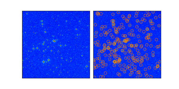
The list x2,y2 has the stars the were found. The rest is image display code to draw circles around the stars and create an image that shows where they are.

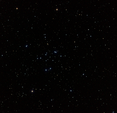
When the program processes a 100 second image of the open cluster M34, shown above, it identifies the stars in the right panel below.

Examples

For examples of Python illustrating image processing, see the examples section.

Assignments

For the assigned homework to use these ideas, see the assignments section.

Image processing with Python and SciPy

Contents

Python Imaging Library - PIL

SciPy image processing

Astronomical FITS files with PyFITS

Displaying a FITS file in Python

Flipping and rotating images

Dark subtraction and flat fielding

FITS headers

Processing images with SciPy

Adding SciKits

Examples

Assignments

Navigation menu

Image processing with Python and SciPy

Python Imaging Library - PIL

SciPy image processing

Astronomical FITS files with PyFITS

Displaying a FITS file in Python

Flipping and rotating images

Dark subtraction and flat fielding

FITS headers

Processing images with SciPy

Adding SciKits

Examples

Assignments

Navigation menu

Search