M15

The globular cluster M15 is very bright, but compact. At a distance of about 33,600 light years it takes a long exposure to capture its faintest stars. This image is a relatively short exposure. It is limited by the brightness of the night sky at our site, by ``seeing'' or atmospheric turbulence, and by the ``less than perfect'' focus (which smears the otherwise point image of a star over several pixels). 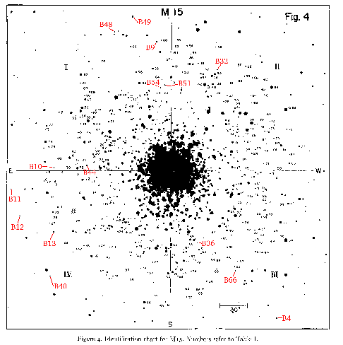Compare this image with the map of M15 in the image file m15_arp1955.jpg. This is a reproduction of a figure published in Color-magnitude diagrams for seven globular clusters, by Halton Arp, Astronomical Journal 60 317 (1955). While the article is an old one, it still provides some of the best available data on the brighter stars of the cluster. This figure labels the individual stars so that you can look up their ``visible'' magnitudes. Although our CCD detector is more sensitive to red light than to blue light, we can approximately compare these photographically measured magnitudes to the unfiltered CCD images. Later, for more precision, we may take images in different colors and measure the color index of each star as well as its magnitude.

Select a 100 second exposuredark-subtracted image of M15 and use the Zoom->Invert Y selection so that north will be at the top. This will help when you compare your image with the map. Use the Scale->Parameters submenu and adjust the lower and upper limits of the signal to show every faint star. The center of the cluster will be saturated and completely white on the screen, but you may adjust the contrast and bias using the Scale->Scale Parameters submenu to make the faint stars clearly visible.

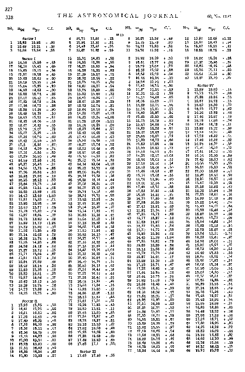
The numbers on the figure refer to entries in the tables. (The stars marked with B are variable.) Notice that the reference map image of M15 is divided into four Roman Numeral sections and that each section has a list of numbered stars in the table. You may read the tables at the computer by using the command

gv m15_tables.ps

but a facsimile is included here too. This image is available in a fits file arp_m15_var.fits that you may display with ds9 for comparison with the images from the telescope.

The visible magnitudes are called $m_{pv}$ where the subscript is for ``photovisual''. Find about 10 stars on the image including some that are very faint and others that are very bright. The range of digital signals from these should span from less than 500 at at the low end to more than 4000 at the high end. Make a table listing the star identification, the photovisual magnitudes ($m_{pv}$) and the measured digital signal from the CCD image ($s$). Also include in your table a column with values of $10^{-2/5(m)}$. You will see why this is useful in just a moment. Use the data in this table to plot graphs with $s$ versus $m$ and $s$ versus $10^{-2/5(m)}$. For this experiment you may do this by hand, but there is powerful software available on these computers called grace or xmgr that is very useful for scientific data analysis. If you want to try that and you are unfamiliar with its use, ask for help.

You will notice in your graph that a larger magnitude means a smaller signal, and also that the relationship is not a linear one. Magnitudes ($m$) arose historically from measurements made visually with the unaided eye. In the present day quantitative form they are a logarithmic scale of luminosity ($\ell$) such that an increase of $5$ in $m$ results from a factor of $100\times$ decrease in $\ell$

$$m - m_0 = -5/2 \cdot \log_{10} (\ell/\ell_0)$$

The CCD should respond with a signal ($s$) linearly proportional to the light received from the star. Ideally, your graph should follow

$$m - m_0 = -5/2 \cdot \log_{10} (s/s_0)$$

where $s_0$ is the signal for a reference magnitude m$_0$. However even for a dark-subtracted image there is a contribution to the signal that does not come from the star. The sky itself creates a signal. This arises from urban light scattered by the lower atmosphere, and from airglow emitted in the upper atmosphere. At our site the scattered urban light, also called light pollution, is very strong. Suppose that the combination of these effects produces a signal $s_{sky}$ in every pixel of the image. If so, then the relationship between stellar magnitude and signal would become

$$m - m_0 = -5/2 \cdot \log_{10} \left(\left(s-s_{sky}\right)/s_0\right)$$

We are free to choose $m_0$, so to make the fitting simple let us take $m_0=0$. The relationship becomes

$$m = -5/2 \cdot \log_{10} \left(\left(s-s_{sky}\right)/s_0\right)$$

or

$$\left(\left(s-s_{sky}\right)/s_0\right) = 10^{-(2/5)m}$$

$$s = s_0 \cdot 10^{-(2/5)m} + s_{sky}$$

Use your data table for M15 and this linear equation between $s$ and $10^{-(2/5)m}$ to find $s_0$ and $s_{sky}$ by fitting a straight line to the graph.

What magnitude corresponds to $s_{sky}$?

Rewrite your solution in this form

$$m = m_0 - 2.5 \cdot \log_{10} (s - s_0)$$

Here $m_0$ is the magnitude that produces a signal of 1 unit above the sky background. With our SBIG ST8E camera $1$ analog-to-digital unit or ADU corresponds to the detection, on the average, of only 2.5 photons. Now by measuring $s$ you may calculate $m$ from this fit to the calibration stars.

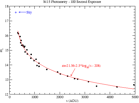
An example of the relationship is shown in this figure, but it may differ from the values for your image.

What do you think the faintest star (highest magnitude) you could measure on this image would be? Why?

Some of the stars in M15 pulsate in brightness with periods from 0.30 to 1.44 days,and a average range from minimum to maximum of about 0.8 magnitudes. Stars that fall in a particular class called RR Lyrae stars (named after a prototype in Lyra) all have about the same physical properties. The absolute magnitude (M) of a star is the magnitude it would have if it were 10 parsecs, about 33 light years, from us. We know from measurements of the statistical properties of the proper motion of nearby RR Lyrae stars that their mean absolute magnitude is about $M=+0.5$ independent of their period of variability. The mean magnitude of an RR Lyrae star, taken as the average of its minimum and maximum magnitude, is also independent of its period. If you know the absolute magnitude of a star, you may use the relationship

$$m-M=5 \log d - 5$$

to find the distance $d$ in parsecs. This equation follows directly from the inverse square law for the flux of light from a distant source and the relationship between magnitude and luminosity.

Which stars in M15 are variable? A sequence of images taken frequently over the course of a night would show them blinking, some from maximum to minimum to maximum again in about 3 hours. If we have such a set, use them to find several RR Lyrae stars. If not, several are marked on the map of M15 with the labels B ... for a catalog made by Solon Bailey in 1919.

Use variable stars you have identified, or a few marked with B on the map. What is the apparent magnitude of these stars? If their average absolute magnitude is $+0.5$, what is the distance of M15 in parsecs?