NumPy, SciPy and SciKits

Python provides a framework on which numerical and scientific data processing can be built. As part of our short course on Python for Physics and Astronomy we will look at the capabilities of the NumPy, SciPy and SciKits packages. This is a brief overview with a few examples drawn primarily from the excellent but short introductory book SciPy and NumPy by Eli Bressert (O'Reilly 2012). The National Radio Astronomy Observatory's Common Astronomy Software site has a helpful introduction to NumPy.

NumPy

NumPy adds arrays and linear algebra to Python, with special functions, transformations, the ability to operate on all elements of an array in one stroke. Remember that in addition to the web resources, in interactive Python try help() for more information on a function:

help("numpy.arange")

will tell you that arange takes one required argument but has several optional ones:

numpy.arange = arange(...)
   arange([start,] stop[, step,], dtype=None
   Return evenly spaced values within a given interval.

Let's see how to create and manipulate arrays with arange and other functions.

Arrays

Arrays are at the heart of NumPy. The program

import numpy as np

mylist = [1, 3, 5, 7, 11, 13]
myarray = np.array(mylist)
print myarray

creates a list and makes an array from it. You can create an array of 30 32-bit floating point zeros with

myarray = np.zeros(30, dtype=np.float32)

The dtype argument is optional (defaults to float64) and can be

• unit8, 16, 32, 64
• int8, 16, 32, 64
• float16, 32, 64, 128
• complex64, 128

Arrays may also have character data, as in this

test = np.array(['a very','friendly','dog'])

which will be a dtype of

test.dtype

dtype('|S8')

meaning a string of 8 characters (set in this instance by the "friendly" element of the list). Arrays must have all elements the same size.

Arrays can be arranged to be multi-dimensional. In our example of zeros, we could instead have

myarray = np.zeros((3,4,5))
print myarray

which will show

array([[[ 0.,  0.,  0.,  0.,  0.],
       [ 0.,  0.,  0.,  0.,  0.],
       [ 0.,  0.,  0.,  0.,  0.],
       [ 0.,  0.,  0.,  0.,  0.]],

      [[ 0.,  0.,  0.,  0.,  0.],
       [ 0.,  0.,  0.,  0.,  0.],
       [ 0.,  0.,  0.,  0.,  0.],
       [ 0.,  0.,  0.,  0.,  0.]],

      [[ 0.,  0.,  0.,  0.,  0.],
       [ 0.,  0.,  0.,  0.,  0.],
       [ 0.,  0.,  0.,  0.,  0.],
       [ 0.,  0.,  0.,  0.,  0.]]])

Notice that the array is created with np.zeros(), and the argument is (3,4,5). This means an array of 3x4x5 elements, all zero (float64, by default), grouped as 3 elements, each of 4 elements, each of 5 elements.

An array can be reshaped after it is made. The array stays the same way in memory, but the grouping changes.

myarray = np.array( [1,3,5,7,11,13] )

makes a linear array of 6 elements, and

myarray.reshape(2,3)
 

changes its shape, so it will be

array([[ 1,  3,  5],
      [ 7, 11, 13]])

To create an array of 1000 elements from 0 to 999, the function

my_1d_array = np.arange(1000)

It is reshaped into an array 10x10x10 with

my_3d_array = my_1d_array.reshape((10,10,10))

or an multi-dimensional array may be flattened

my_new_array = my_3d_array.ravel()

The original data remain unchanged, but they are sliced and indexed in different ways depending on the shape of the array and the choices for indexing it.

In summary, NumPy arrays may be created with

 np.array()
 np.arange()
 np.zeros()
 np.empty()

reshaped with

 myarray.reshape()
 myarray.ravel()

written to files in a binary format, and read back with

 np.save('myfile.npy', myarray)
 newarray = np.load('myfile.npy')

In the following we will see how to index within arrays, operate on arrays, and have arrays functionally combine with one another.

Indexing

Once an array is created, you can refer to it as a whole, or to its elements one-by-one. Create a list, turn it into an array, reshape it, and print it with something like this

#Make a list
mylist = [1,2,3,4,5,6,7,8,9,10,11,12]

#Make an array from a list
myarray = np.array(mylist)

#Reshape the array
my3by4 = myarray.reshape(3,4)
print my3by4

to see

array([[ 1,  2,  3,  4],
      [ 5,  6,  7,  8],
      [ 9, 10, 11, 12]])

The (2,3) element in the reshaped array is

print my3by4[2][3]

12

Remember that indexing is from 0, so the "2" here means the 3 "group", and each group had 4 elements. The "3" means the fourth element of that group, which is 12.

Therefore, the notation is just like matrices, with the first index the row and the second index the column, enumerated from (0,0) at the upper left as printed.

Lists in Python are indexed similarly. Make a grouped list this way

alist = [[2,4],[6,8]]
print alist[0][1]

displays

4

as expected. With NumPy you can also get access to a selected column --

arr = np.array(alist)
print arr[0][1]

shows "4". The way to have column 1 alone is

print arr[:,1]

shows us a list of column 1,

[4 8]

and

print arr[1,:]

shows the list of row 1,

[6 8]

It's also possible to find elements conditionally. Let's make an array of 16 elements from 0 to 15, shape it to 4x4, and find those elements greater than 5

# Create the array 
myarray = np.arange(16).reshape(4,4)
print myarray 

array([[ 0,  1,  2,  3],
      [ 4,  5,  6,  7],
      [ 8,  9, 10, 11],
      [12, 13, 14, 15]])

# Index the array
myindex = np.where(myarray <5)
print(myindex)

(array([0, 0, 0, 0, 1]), array([0, 1, 2, 3, 0]))

mynewarray = myarray[myindex]
print mynewarray

array([0, 1, 2, 3, 4])

Functions Broadcasting Over an Array

The term broadcasting in NumPy refers to applying an operation to every element of an array. Consider this simple example

cube = np.zeros((2,2,2))

that makes a 2x2x2 cube of zeros. You can add 1 to every element, then divide them all by 3, with

newcube = (cube + 1.)/3.
print newcube

array([[[ 0.33333333,  0.33333333],
       [ 0.33333333,  0.33333333]],

      [[ 0.33333333,  0.33333333],
       [ 0.33333333,  0.33333333]]])

Perhaps more interestingly, create an array of multiples of Pi with

manypi = np.arange(8)*np.pi/4.

and then find the sine of these angles

manysines = np.sin(manypi)

The first one will produce the array of angles

array([ 0.        ,  0.78539816,  1.57079633,  2.35619449,  3.14159265,
       3.92699082,  4.71238898,  5.49778714])

and the second will give the array of their sines

array([  0.00000000e+00,   7.07106781e-01,   1.00000000e+00,
        7.07106781e-01,   1.22464680e-16,  -7.07106781e-01,
       -1.00000000e+00,  -7.07106781e-01])

NumPy math has the usual trigonometric functions, and others. A full list is in the documentation, and some useful ones are for element-by-element

• add(x1,x2)
• sub(x1,x2)
• multiply(x1,x2)
• divide(x1,x2)
• power(x1,x2)
• square(x)
• sqrt(x)
• exp(x)
• log(x)
• log10(x)

• absolute(x)
• negative(x)

• sin(x), cos(x), tan(x)
• arcsin(x), arccos(x), arctan(x)
• arctan2(x,y) returns the angle whose tangent is the ratio of x and y
• sinh(x), cosh(x), tanh(x)
• arcsinh(x), arccosh(x), arctanh(x)

• degrees(x) or rad2deg(x) convert from radians
• radians(x) or deg2rad(x) convert from degrees

• rint(x) round to the nearest integer
• fix(x) round to the nearest integer toward zero

The broadcast feature of NumPy arrays can be combined with selective indexing in an interesting way. Consider this program to make an array of random numbers in a Gaussian distribution with mean 0, and sigma 1

a = np.random.randn(100)

Print this will show 100 values, some negative, some positive. We can select only those larger than a cutoff, work with them, and put them back in the array

index = a > 0.75
b = a[index]
b= b ** 3 - 100.
a[index] = b

Printing index will show an array of True and False that mask the original array. The array b will only have those elements that satisified the condition used to make the index. The index is used again, to put modified elements back into the original array.

Matrix and Vector Math in NumPy

We have seen that NumPy has its own set of math functions that broadcast over arrays. If you define an array

a = np.arange(0,1,0.01)*np.pi

you will have an array from 0 to Pi in steps of 0.01*Pi. You can operate on this array, element by element, with np.cos

b = np.cos(a)

and have a new array that contains the cosine of each element of the first one.

Before we move on to SciPy, which builds on NumPy to add a number of useful features, there are two things we should note.

First, NumPy includes matrix math, either by mapping its native arrives to conventional matrices, or by invoking matrix math operations on its arrays. We will only look at this second way, which handles most applications and creates very clear code.

The product of two matrices is done with the "dot" operation between two NumPy arrays.

a = np.array(([1,2],[3,4]))
b = np.array(([0,1],[1,0]))

makes two arrays that may be thought of as 2x2 matrices. To multiply them in the usual sense of matrix multiplication,

c = a.dot(b)

gives

array([[2, 1],
      [4, 3]])

and

d = b.dot(a)

gives

array([[3, 4],
      [1, 2]])

A matrix inverse is found in the linalg package of NumPy

e = np.linalg.inv(a)

With this we can solve linear equations. Suppose that you have the system of 3 equations in 3 unknowns:

2x + y = 1
3y + z = 1
x + 4z = 1

We would write

a = np.array([[2, 1, 0], [0, 3, 1], [1, 0, 4]])
b = np.array([[1],[1],[1]])

The linear algebra formulation is a.X = b, with solution X = a^-1 . b where a^-1 is the inverse of a. In NumPy we would find

x = np.linalg.inv(a).dot(b)
print x

which as a program returns the solution

array([[ 0.36],
      [ 0.28],
      [ 0.16]])

NumPy also supports vector math with np.cross. For example if

a = [1, 1, 0]
b = [0, 0, 1]
c = np.cross(a, b)
print c

array([ 1, -1,  0])

d = np.dot(a, b)
print d

0

Or, to illustrate the dot product in another example

a = np.array([1,0,0])
b = np.array([2,1,3])
d = np.dot(a,b)
print d

2

For 1-D vectors this is the same as the inner product

d = np.inner(a,b)
print d

2

Fourier Transforms in NumPy

NumPy provides Fourier Transforms in several functions, including the one-dimension discrete Fast Fourier Transform or FFT with the function fft(a), and the one-dimensional FFT of real data with rfft(a). It also has n-dimensional Fourier Transforms as well.

As a very simple example, let's consider an exponential decay modulating a sine wave adapted from our dampled cosine plotting example to use NumPy arrays:

# Import the plotting and math packages
import matplotlib.pyplot as plt
import numpy as np

# Define initial constants
f0 = 5.
a0 = 100.
tdecay = 2.
timestep = 0.01
timemax = 100.

time = np.arange(0,timemax,timestep)
amplitude = np.exp(-time/tdecay)*np.cos(2.*np.pi*f0*time)

With NumPy we do not have to loop to calculate each point of the damped oscillator's path.

Now we add a Fourier Transform with lines

# Use an FFT to calculate its spectrum
spectrum = np.fft.fft(amplitude)

# Find the positive frequencies
frequency = np.fft.fftfreq( spectrum.size, d = timestep )
index = np.where(frequency >= 0.)

# Scale the real part of the FFT and clip the data
clipped_spectrum = timestep*spectrum[index].real
clipped_frequency = frequency[index]

The array "spectrum" has the spectrum of the original data, and "frequency" has the corresponding frequencies. We clip the negative frequencies.

# Create a figure
fig = plt.figure()

# Adjust white space between plots
fig.subplots_adjust(hspace=0.5)

# Create x-y plots of the amplitude and transform with labeled axes

data1 = fig.add_subplot(2,1,1)
plt.xlabel('Time')
plt.ylabel('Amplitude')
plt.title('Damping')
data1.plot(time,amplitude, color='red', label='Amplitude')
plt.legend()
plt.minorticks_on()
plt.xlim(0., 10.)

data2 = fig.add_subplot(2,1,2)
plt.xlabel('Frequency')
plt.ylabel('Signal')
plt.title('Spectrum of a Damped Oscillator')
data2.plot(clipped_frequency,clipped_spectrum, color='blue', linestyle='solid', 
 marker='None', label='FFT', linewidth=1.5)
plt.legend()
plt.minorticks_on()
plt.xlim(3., 7.)

# Show the data
plt.show()

This will make an interactive plot that looks like this

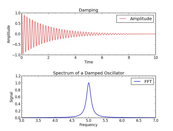
In practical applications it is desirable to have programs that will read files containing time or frequency data, perform the Fourier transform, and export a file with the transform from frequency to time, or from time to frequency. Two programs that are useful in this way are included in the examples section. They depend on SciPy, which is described in the following.

• fft_f2t.py
• fft_t2f.py

SciPy and SciKits

NumPy adds numerical support to Python that enables a broad range of applications in science in engineering. SciPy and SciKits use NumPy to provide features that are targeted at scientific computing. These packages are dynamic, with community support that is adding new contributions and updating older ones. As we continue our short course on Python for Physics and Astronomy we will explore a few of these to see how we can use Python for interpolating data, numerical integration, and image processing. A reference guide to SciPy is available on line from the their website, or in this reference pdf if that site is not available.

Interpolation

Frequently we will have data that are not as finely spaced as we would like, but which are smooth enough to reliably interpolate between the known points. An example might be a resource-intensive computation of a wavefunction for a complex system, a model of the opacity of stellar atmosphere, or a calculation of of a planetary atmosphere on a coarse spatial grid. You can also interpolate noisy data and recover an acceptable estimate of the values between the sampled points.

For example, this program will create a set of test data of a sparsely sampled cosine curve, and then fit it with a linear and a quadratic approximation.

import numpy as np
from scipy.interpolate import interp1d
import matplotlib.pyplot as plt

# Import your data into a np array yn for x or ...

# Generate sample data
x = np.linspace(0,10.*np.pi,200)  
y = np.cos(x)

# Function to interpolate the data with a linear interpolator
f_linear = interp1d(x, y, kind='linear')

# Function to interpolate the data with a quadratic interpolator
f_quadratic = interp1d(x, y, kind='quadratic')

# Values of x for sampling inside the boundaries of the original data
x_interpolated = np.linspace(x.min(),x.max(), 1000)

# New values of y for these sample points
y_interpolated_linear = f_linear(x_interpolated)
y_interpolated_quadratic =  f_quadratic(x_interpolated)

It helps to plot this

# Create an plot with labeled axes
plt.xlabel('X')
plt.ylabel('Y')
plt.title('Sample Interpolation')
plt.plot(x, y,   color='red', linestyle='None', 
 marker='.', markersize=10., label='Data')
plt.plot(x_interpolated, y_interpolated_linear, color='green', linestyle=':', 
 marker='None', label='Linear', linewidth=1.5)
plt.plot(x_interpolated, y_interpolated_quadratic, color='blue', linestyle='-', 
 marker='None', label='Quadratic', linewidth=1.5)
plt.legend()
plt.minorticks_on()
plt.show()

The result, zoomed in to see a few points in detail, looks like this on an interactive screen:

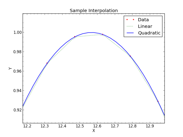
For 1-dimensional interpolation we have tried "linear" and "quadratic" which have clear meanings. The linear interpolation does a linear fit between two adjacent points and uses that to find the value at an x between those points. As you can see in the graph, the values follow a straight line connecting the sample points. The quadratic interpolator takes points bracketing the x of interest and fits a quadratic polynomial to them. This allows the interpolation to have non-zero second derivative, and visually the new data will "curve" between the original sample points.

The choices available for "kind" include

• linear
• quadratic
• cubic
• 1,2,3, or higher indicating order of spline

When the data support it, cubic interpolation introduces a third derivative, and gives a better representation of the original. You would not use linear interpolation of position to find velocity, and if you wanted to know the rate of change of acceleration you might use cubic interpolation.

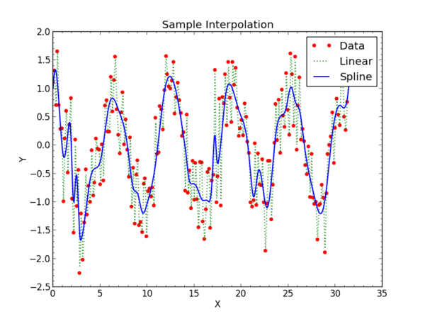
For more functions where the shape is not well represented by a polynomial, a spline fit will adapt to the available points and give a representation of the data better than fixed polynomials. The cubic spline is the most often used. Another implementation of spline fitting comes is incorporated into SciPy's UnivariateSpline function.

Similar to the fitting above, the program to use spline fitting would have lines such as these

from scipy.interpolate import UnivariateSpline 

# Generate sample xdata
x = np.linspace(0,10.*np.pi,200)  

# Add noise to the sample y-data
y = np.cos(x)+ 0.5 * np.random.normal(size=len(x))

# Function to interpolate the data with a univariate spline interpolator
f_spline = UnivariateSpline(x, y, k=3, s=40)

# Values of x for sampling inside the boundaries of the original data
x_interpolated = np.linspace(x.min(),x.max(), 1000)

# New values of y for these sample points
y_interpolated_spline =  f_spline(x_interpolated)

The function call to UnivariateSpline uses an optional smoothing factor argument "s=40". If "s=0" the spline will interpolate through all the points. The larger this value, the more the spline filters short interval changes. Another optional argument is the order of the smoothing spline which is specified with "k=3". It must be less than or equal to 5.

The complete program is in the Examples section. It will create a new data and a different fit on each run because it calls a random number generator.

Integration

The SciPy integrate module supports numerical integrating a function of 1 to 3 variables, and integrating numerical data using trapezoidal, Simpson's rule, and Romberg methods. It also supports integrating ordinary differential equations.

import scipy.integrate
help("scipy.integrate")

   Integrating functions, given function object
   ============================================
       
      quad          -- General purpose integration.
      dblquad       -- General purpose double integration.
      tplquad       -- General purpose triple integration.
      fixed_quad    -- Integrate func(x) using Gaussian quadrature of order n.
      quadrature    -- Integrate with given tolerance using Gaussian quadrature.
      romberg       -- Integrate func using Romberg integration.
   
  Integrating functions, given fixed samples
   ==========================================
       
      trapz         -- Use trapezoidal rule to compute integral from samples.
      cumtrapz      -- Use trapezoidal rule to cumulatively compute integral.
      simps         -- Use Simpson's rule to compute integral from samples.
      romb          -- Use Romberg Integration to compute integral from
                    -- (2**k + 1) evenly-spaced samples.

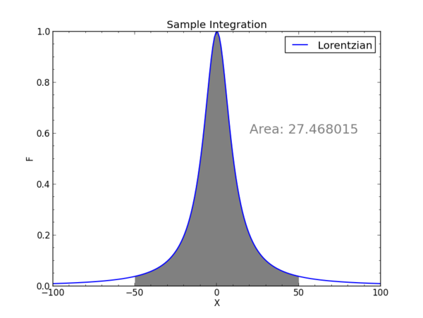
As first example of integrating a function we will try a Lorentzian curve

import numpy as np
from scipy.integrate import quad
import matplotlib.pyplot as plt

# Define the integrand

global a
a = 10.
f = lambda x: a**2 / (a**2 + x**2)

x0 = -50.
x1 = 50.

integral, error = quad(f, x0, x1)

# Compare integral to an area under the curve out to infinity

area = a * np.pi
print integral, area

which we will plot in a moment. As is, it will print the integral from -50 to 50 under the Lorentzian curve (generated with the "f" definition) and a=10. As given, this Lorentzian has a peak of 1, and it falls to 0.5 of the peak at x=a. The area is exactly a x Pi.

You can iterate this by hand and see that as the limits are extended to infinity the integral slowly converges to the exactly value it would have at infinite limits. You can also generate a numerical infinity by using

x0 = -np.inf
x1 = np.ing

A helpful plot can be made by adding this code:

# Generate sample data
x = np.linspace(-100,100.,200)  
y = f(x)

# Create an integration region to show in the plot
index01 = np.where( (x > x0) & (x < x1) )
y_region = y[index01]
x_region = x[index01]

# Create a plot with labeled axes
plt.xlabel('X')
plt.ylabel('F')
plt.title('Sample Integration')
plt.plot(x, y, color='blue', linestyle='-', marker='None',
  label='Lorentzian',linewidth=1.5)
plt.fill_between(x_region, 0., y_region, color='gray')
plt.legend()
plt.minorticks_on()

# Annotate with area
area_label = 'Area: %f' % integral
print area_label
plt.annotate(area_label, xy= (.6,.6), xycoords='axes fraction', 
  color='gray', fontsize=18)
plt.show()

With this you will see a graph of the function and the area being integrated.

Numerical integration would go similarly, except the input would be numpy arrays for x and y from data points or generated this way

import numpy as np
from scipy.integrate import trapz
import matplotlib.pyplot as plt

# Define the integrand

global a
a = 10.

def f(x):
  value = a**2 / (a**2 + x**2)  
  return value

# For a good demonstration use
x0 = -50.
x1 = 50.

x = np.linspace(x0,x1,1000)
y = f(x)

integral = trapz(y, x=x)

Differentiation

SciPy provides differentiation of functions, much in the same fashion as it offers integration.

derivative(func, x0, dx=1.0, n=1, args=(), order=3)

where the "func" is the function being differentiated at "x0", "dx" is the interval on x used to find the derivative, "n" is order for the differentiation (by default 1 for first derivative), and "order" is the number of points to use in finding the derivative, not to be confused with the order of the differentiation. The "args" argument allows a function to call other arguments, rather than have them globally defined as we do in these examples.

An example of its use to find the first derivative

import numpy as np
from scipy.misc import derivative

# Define the function
def f(x):
  value = x**2 * np.exp(-(x**2)) 
  return value

result = derivative(f, 1., dx=0.01)
print result
2.452186e-05

result = derivative(f, 2., dx=0.01)
print result
-0.21979

The result can be very sensitive to the choice of dx, which must be small enough to see the representative incremental changes.

Differentiation of NumPy arrays can be done without additional programming, since it is only the difference between uniformly spaced values. However, for noisy data it would be best to interpolate the data first, and then take differences between adjacent points to calculate the derivative. Given the arrays, the derivative might be found with

 np.diff(y) / np.diff(x)

with suitable tests for pathological behavior.

In some cases it is possible to use symbolic analytic differentiation with the SymPy package that has evolved into a robust full-featured symbolic mathematics tool.

Statistics

As expected, SciPy provides statistical functions to Python in the form of various conventional statistical discrete and continuous distributions. The normal distribution is first one we would usually encounter:

import numpy as np
from scipy.stats import norm

# Create a sample sapce
x = np.linspace (-10,10,1000)

# Set up the parameters of the distribution
# Here loc makes it center on the origin and scale gives unit scaling
dist = norm(loc=0, scale=1)

# Now find the probability density function or pdf
pdf = dist.pdf(x)

# Plot the result ...

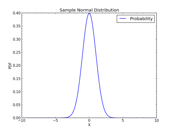
For the normal or Gaussian distribution, we would have

N(x) = (1 / sigma sqr(2 pi) ) exp ( - (x - mu)^2 / 2 sigma^2 )

where sigma is the standard deviation, sigma^2 is the variance, and mu is the mean. The factor in front normalizes the distribution to unit area integrated to infinity on x. A Gaussian distribution centered at the origin has mu=0 and a width such that at x=sqr(2)sigma the distribution is 1/e of its maximum at x=0.

Numpy would also allow creating a normal random array of values with mean 0 and variance 1, such as

y = np.random.randn(1000)

The mean, standard deviation, and variance could be assessed by evaluating the array

mean = y.mean()
std =  y.std()
var = y.var()

SciKits Packages

We mention SciKits in the context of SciPy because it is a collection of SciPy applications that extend into many different domains of physics, astronomy, and engineering. The best introduction is to browse the SciKits website and explore the variety there. In addition to image processing, you'll find speech processing, light scattering from non-spherical particles, sparse matrices, machine learning, vector field plotting, and more. Some are fully developed, others are works in progress. One of the most promising is the scikits.cuda package, which interfaces Python to CUDA, NVidia's parallel processing through graphical processing units (GPU). The most recent hardware at this date (February 2017), is the the Tesla P100 Pascal architecture for servers, a supercomputer on a PCIe card with 3584 GPU cores, 9.3 Teraflops of single precision and 4.7 Teraflops of double precision processing power, and 16384 MB of memory.

An example of a very useful Scikit is the image restoration package which includes Lucy-Richardson deconvolution. A program that makes use of it for astronomical fits images is in the examples directory of this site. Look for fits_lucy_richardson.py under the convolution examples.

We will return to use other SciPy image processing routines later.

Examples

For examples of NumPy and SciPy, see the examples section. Look for

• curve_fit_plot.example
• integrate_function_plot.example
• integrate_numerical_plot.example
• interpolate_noisy_plot.example
• interpolate_plot.example
• norm_probability_plot.example
• numpy_fft.example
• fft_f2t.py
• fft_t2f.py

that contain most of the code shown in this section.

Assignments

For the assigned homework to use these ideas, see the assignments section.